ggplot2
We will use the mtcars dataset, which comes pre-loaded in the R session. Explore the dataset by executing str(mtcars) and summary(mtcars) in the R console.
Note
You can download the full R Script to reproduce the analysis here.
Load the ggplot2 package using:
library(ggplot2)
Scatterplots
Plotting with base R:
plot(mtcars$hp,mtcars$mpg)
Plotting with ggplot2:
scatterplot <- ggplot(mtcars, aes(x = hp,y = mpg)) +
        geom_point()
Add axis titles:
scatterplot <- scatterplot +
  labs(title = "MPG vs HP",
       x = "HP",
       y = "Miles Per Gallon")
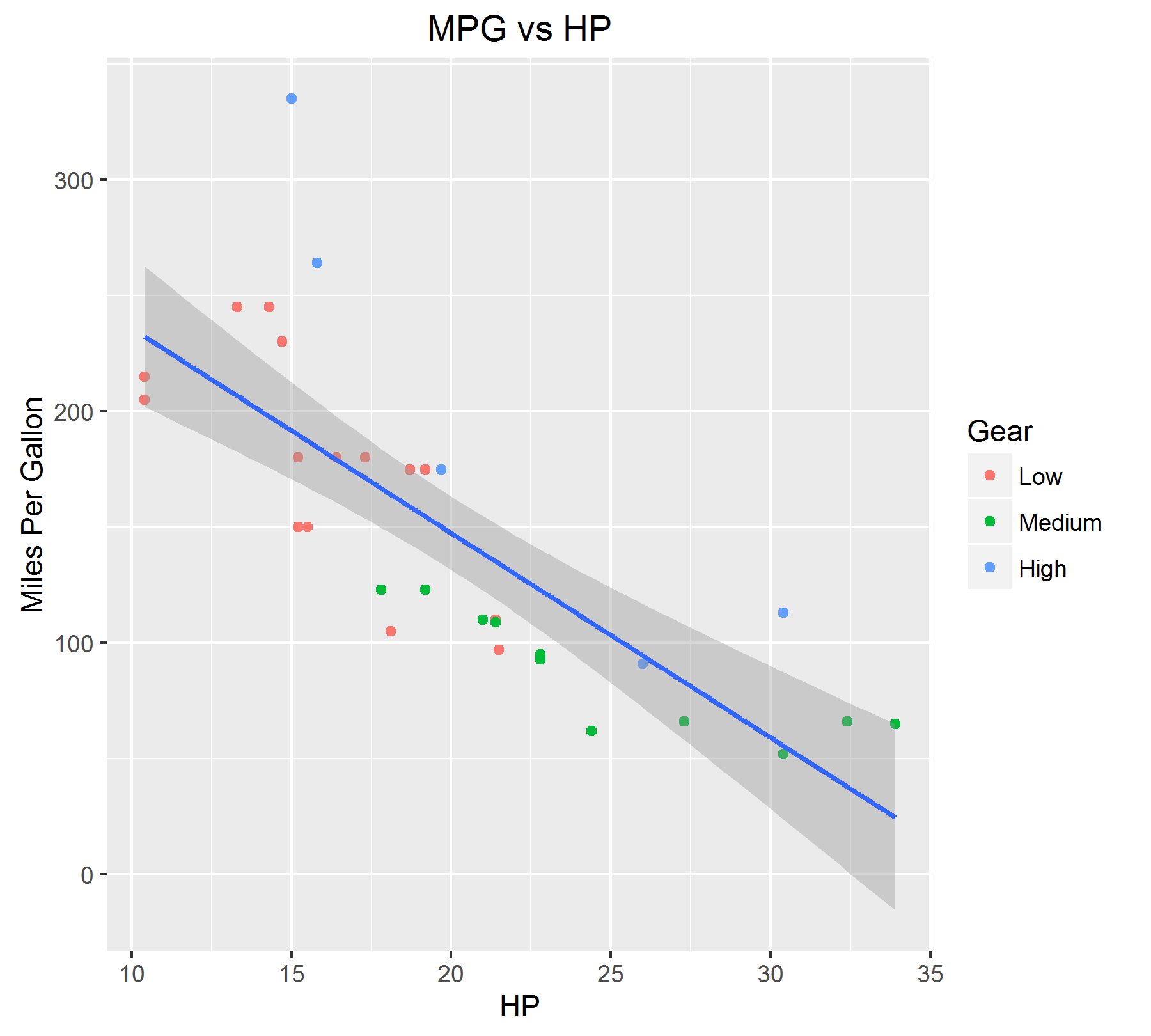
Make legend discrete, and add regression line for final graph:
mtcars$gear <- as.factor(mtcars$gear)

scatterplot <- ggplot(mtcars, aes(x = mpg,y = hp)) +
  geom_point(aes(colour = mtcars$gear)) +
  geom_smooth(method = "lm",se = FALSE) +
  scale_colour_discrete(name = 'Gear',
                        breaks = c('3','4','5'),
                        labels = c('Low','Medium','High')) +
  labs(title = "MPG vs HP",
       x = "HP",
       y = "Miles Per Gallon")
Histograms
ggplot(mtcars, aes(x = mpg)) +
  geom_histogram(binwidth = 5)
Make the graph pretty:
ggplot(mtcars, aes(x = mpg)) +
  geom_histogram(binwidth = 5,
                 colour = "black",
                 fill = "white") +
  labs(title = "Distribution - Miles Per Gallon",
       x = "Miles Per Gallon",
       y = "Count")
Saving your graphs
?ggsave gives you a description of the parameters that the function takes, and their defaults:
ggsave(filename, plot = last_plot(), device = NULL, path = NULL,
        scale = 1, width = NA, height = NA, units = c("in", "cm", "mm"),
        dpi = 300, limitsize = TRUE, ...)
To save our scatterplot, we might want to use the following parameters:
ggsave(filename = 'FULL_FILE_PATH.FILE_TYPE',
        plot = scatterplot,
        width = 6,height = 5.4)
FILE_TYPE can be tex, pdf, jpeg, png, svg and others (refer documentation by using ?ggsave).
Output